Background:

In this tutorial, We plan to extract the raster cell values from the set of point features nd records the values in the attribute table as an output. on Google Earth Engine (GEE) with python API. Before we dive into the working steps, I will explain the general idea of how this concept can be implemented. 
The process of raster value extraction can be implemented in two ways, 

• Directly extracting the raster values by overlaying raster with point data. Raster value which perfectly overlays with the point is taken.
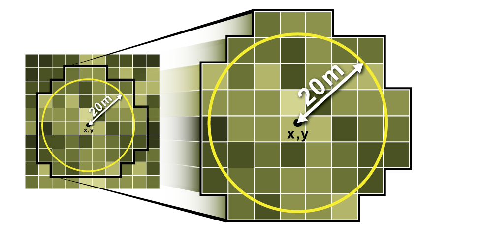
• Buffer (circle, square) around the point is created, and raster statistics (mean) are obtained. This mean is taken as the raster value for points. Refer this: 
• 

Scenario, where you are going to need raster value extraction:

At some point, anyone working with field data collected in plots will almost certainly need to extract raster data for those plots. For example, the Normalized Difference Vegetation Index (NDVI) is a widely used measure of vegetation greenness that can be derived using a number of satellite datasets. You might also want to plot climate data or extract reflectance from multispectral satellite bands to compute your own indices later. This method can be used on a single image or a collection of images. When you run the procedure across an image collection, you'll get a table with values from each image per point. Before extraction, Image collections can be treated as appropriate, such as masking clouds from satellite imagery.

Now Let's move into the steps, where the concept is implemented.

Implementation of raster value extraction from points on Google Earth Engine (GEE):

1. Importing modules 

   # import Google earth engine module
   import ee
   
   #Authenticate the Google earth engine with google account
   # First firt setup only, no need to run this after first run
   
   
   # ee.Authenticate()
   
   # for normal/regular use for authorization
   # this is required regularly
   ee.Initialize()
   
   
   #Pandas modules to interact data
   import numpy as np
   import pandas as pd

2. Define indicators of your interest. For this blog, i will demonstrate NDVI and EVI for Sentinel-2 image

   # compute NDVI from NIR and red band in sentinel -2 image
   # For other satellite image, please change the band information accordingly
   
   def getNDVI(image):
       
       # Normalized difference vegetation index (NDVI)
       ndvi = image.normalizedDifference(['B8','B4']).rename("NDVI")
       image = image.addBands(ndvi)
   
       return(image)
   
   
   # compute EVI from NIR and red band in sentinel -2 image
   # For other satellite image, please change the band information accordingly
   
   def getEVI(image):
       # Compute the EVI using an expression.
       EVI = image.expression(
           '2.5 * ((NIR - RED) / (NIR + 6 * RED - 7.5 * BLUE + 1))', {
               'NIR': image.select('B8').divide(10000),
               'RED': image.select('B4').divide(10000),
               'BLUE': image.select('B2').divide(10000)
           }).rename("EVI")
   
       image = image.addBands(EVI)
   
       return(image)

3. Date parameter for image
   It is most important part for time series study.

   # manage the date formating as per your requirements
   # Mine is in format of YYYYMMdd
   def addDate(image):
       img_date = ee.Date(image.date())
       img_date = ee.Number.parse(img_date.format('YYYYMMdd'))
       return image.addBands(ee.Image(img_date).rename('date').toInt())

4. Filter the imagery for your desired timeframe and other parameters
   I have limited the filters for sample only.

   Sentinel_data = ee.ImageCollection('COPERNICUS/S2') \
       .filterDate("2021-01-01","2021-08-31") \
       .map(getNDVI).map(getEVI).map(addDate)

5. Import your point samples here.
   Modify as per your requirements.

   plot_df = pd.read_excel('data/sample_plot_points_random.xlsx')
   plot_df

6. Convert the pandas dataframe into Google Earth Engine (GEE) Feature Collection

   features=[]
   for index, row in plot_df.iterrows():
   #     print(dict(row))
   #     construct the geometry from dataframe
       poi_geometry = ee.Geometry.Point([row['longitude'], row['latitude']])
   #     print(poi_geometry)
   #     construct the attributes (properties) for each point 
       poi_properties = dict(row)
   #     construct feature combining geometry and properties
       poi_feature = ee.Feature(poi_geometry, poi_properties)
   #     print(poi_feature)
       features.append(poi_feature)
   
   # final Feature collection assembly
   ee_fc = ee.FeatureCollection(features) 
   ee_fc.getInfo()

7. Extract the raster values for each features 
   We will use sampleRegions function from ee.image and apply to image collection

   def rasterExtraction(image):
       feature = image.sampleRegions(
           collection = ee_fc, # feature collection here
           scale = 10 # Cell size of raster
       )
       return feature
   

8. Apply raster extraction functions over image collection
   sampleRegions returns feature collection with image values, then we have collection of feature collection which is then flattened to obtain final feature collection. Finally feature collection is converted to CSV. 

   results = Sentinel_data.filterBounds(ee_fc).select('NDVI', 'EVI').map(addDate).map(rasterExtraction).flatten()

9. Verify that output is as per your requirments

   sample_result = results.first().getInfo()
   sample_result

10. Now we have extracted the raster values, We need to convert feature collection to CSV format.
    We can acheive this in multiple ways, I will illustrate in 3 ways for extraction. 

    # extract the properties column from feature collection
    # column order may not be as our sample data order
    columns = list(sample_result['properties'].keys())
    print(columns)
    
    
    # Order data column as per sample data
    # You can modify this for better optimization
    column_df = list(plot_df.columns)
    column_df.extend(['NDVI', 'EVI', 'date'])
    print(column_df)
    
    

11. Method 1: Feature collection to pandas dataframe 

    nested_list = results.reduceColumns(ee.Reducer.toList(len(column_df)), column_df).values().get(0)
    data = nested_list.getInfo()
    data
    
    # dont forget we need to call the callback method "getInfo" to retrieve the data
    df = pd.DataFrame(data, columns=column_df)
    # we obtain the data frame as per our demand
    df

12. Method 2: Direct download Feature collection to CSV via URL link

    url_csv = results.getDownloadURL('csv')
    # click the link below, this will download CSV directly to your local device
    # You can use this url and download with python request module, I will leave that to you
    url_csv
    

13. Method 3: Download feature collection as CSV to Google Drive

    task = ee.batch.Export.table.toDrive(**{
      'collection': results,
      'description':'vectorsToDriveExample',
      'fileFormat': 'csv'
    })
    task.start()
    
    import time
    while task.active():
      print('Polling for task (id: {}).'.format(task.id))
      time.sleep(5)

14. Data visualization of results:
    I will go on details for visualization on the next blog post. 

    # import libraries
    
    # Using plotly.express
    import plotly.express as px
    
    # I will plot line plot for single point only for now.
    # I will cover detail analaysis in next plot
    df_filtered = df[df['id']==1]
    df_filtered['date'] = pd.to_datetime(df_filtered['date'], format='%Y%m%d')
    df_filtered

15. df = px.data.stocks()
    fig = px.line(df_filtered, x='date', y="EVI")
    fig.show()
    
    
    df = px.data.stocks()
    fig = px.line(df_filtered, x='date', y="NDVI")
    fig.show()

Here's some sample for the visualized data. This chart data are highly affected by the cloud cover as I have taken all sentinel -2 data without any cloud mask.

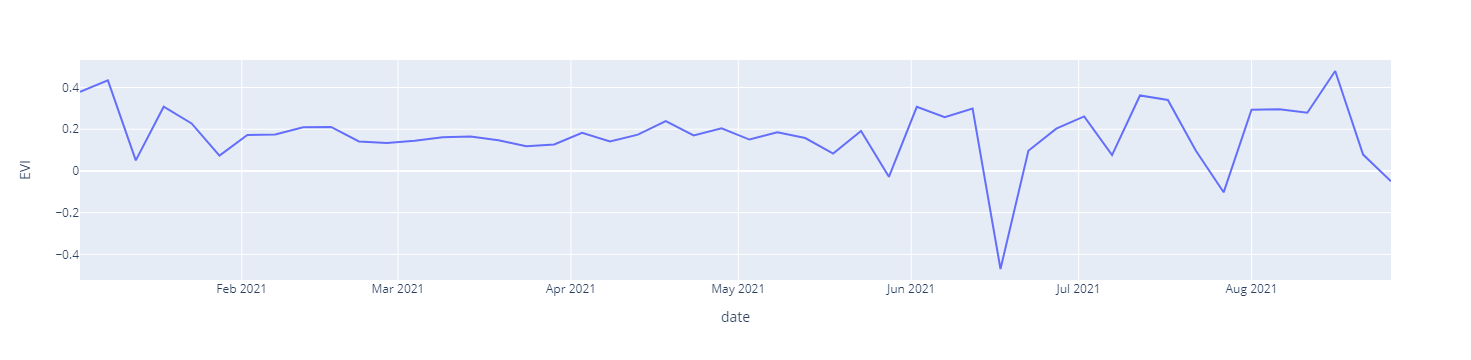
EVI vs Date

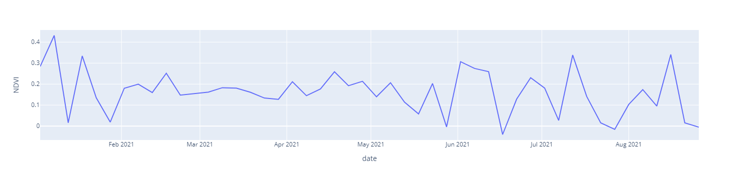NDVI vs Date

Source code: github_link

I will be bringing next post on details for the time series analysis of various vegetation indices.

Please let us know your thoughts on this with following comment section we will definetly reach out to you on your query and feedback.